Embeddings and vector search, explained

An embedding is a vector of numbers that encodes the meaning of a text: two semantically close sentences produce close vectors, even with no shared words. That is what enables semantic search (by meaning) as opposed to keyword search. This article explains what an embedding is, how it's learned, how proximity is measured, and how to scale up with vector search.

What is an embedding?

An embedding is a learned numerical representation that places text (word, sentence, document) in a vector space where geometric proximity reflects semantic proximity. A model converts text of any length into a fixed-size dense vector — e.g. 384 dimensions for all-MiniLM-L6-v2, 1024 for Cohere v3, 3072 for OpenAI text-embedding-3-large.

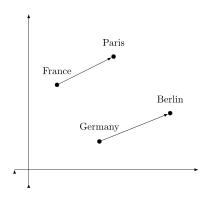Figure: a word embedding. Source: Wikimedia Commons (CC BY-SA).

Unlike sparse lexical representations (bag-of-words, TF-IDF), embeddings place synonyms near each other even with no shared word — the whole difference between "semantic" and "keyword."

How embeddings are learned

The historical line runs from distributional semantics (Firth, 1957) to word2vec (Mikolov et al., Google, 2013), the breakthrough that made word vectors mainstream. word2vec uses a sliding context window with two architectures: CBOW (context predicts the word, faster) and skip-gram (word predicts the context, better for rare words). These vectors are static (one word = one vector).

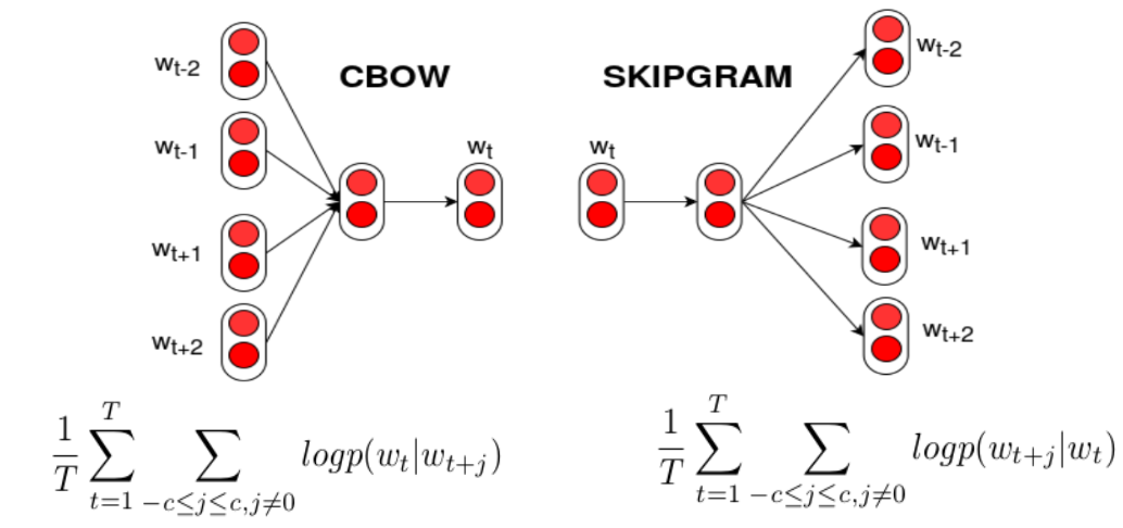Figure: CBOW vs Skip-gram. Source: Wikimedia Commons (CC BY-SA).

Modern sentence embeddings use a bi-encoder trained with a contrastive objective: pull matching (positive) pairs together, push negatives apart. The dominant production loss is MultipleNegativesRankingLoss (in-batch negatives). Finally, contextual models (BERT and successors) give a word a different vector per context, solving polysemy — a key advance over static vectors.

The vector space and the geometry of meaning

Each dimension is a latent feature; meaning is encoded by direction and relative position, not by any single interpretable axis. The linear-analogy structure is famous:

vector("king") − vector("man") + vector("woman") ≈ vector("queen")

The same conceptual offset (royalty) is a consistent direction. You recover the word whose vector has the highest cosine similarity to b − a + c. Since these spaces have hundreds of dimensions, we project to 2-D (t-SNE, UMAP) to visualize clusters.

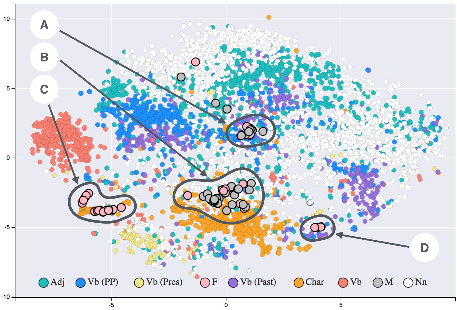Figure: t-SNE projection of embeddings. Source: Wikimedia Commons (CC BY-SA).

Measuring proximity

Similarity is most often measured by the cosine of the angle between two vectors: near 1, meanings are alike; near 0, independent.

function cosine(a: number[], b: number[]): number {
  let dot = 0, na = 0, nb = 0;
  for (let i = 0; i < a.length; i++) {
    dot += a[i]! * b[i]!; na += a[i]! ** 2; nb += b[i]! ** 2;
  }
  return dot / (Math.sqrt(na) * Math.sqrt(nb));
}

The dot product accounts for both direction and magnitude (and is faster); on normalized vectors (unit length), dot product and cosine coincide exactly, and Euclidean distance gives the same ranking. Practical rule: use the metric the model was trained with, normalize end to end, and "if in doubt, pick cosine." A normalization mismatch (normalized index, raw query) silently corrupts ranking.

Vector search and ANN

Comparing the query to every vector (exact kNN) gives 100% recall but costs O(N·d) — untenable at millions of vectors. ANN (Approximate Nearest Neighbors) indexes trade a little exactness for large speed/memory gains. The central trade-off is recall ↔ latency ↔ memory, tuned by parameters.

• HNSW: a multi-layer small-world graph. Search starts at a top entry point, hops to closer neighbors, then descends from coarse to fine layers. Parameters: M (neighbors per node) and ef (search breadth) — higher = better recall, costlier.
• IVF: partition into nlist cells (k-means) and probe only nprobe cells per query.
• PQ / quantization: split a vector into subvectors replaced by centroid IDs — up to ~64× compression, at a recall cost to watch.

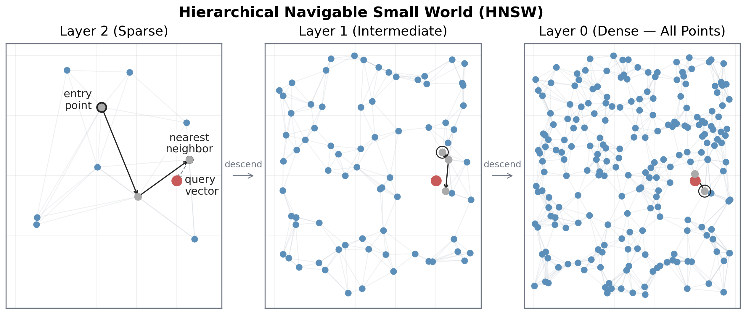Figure: HNSW index. Source: Wikimedia Commons (CC BY).

Vector databases

A vector DB stores embeddings + metadata and serves low-latency ANN queries at scale (pgvector, Qdrant, Weaviate, Pinecone; with FAISS as the underlying index library). Key features: ANN index, metadata filtering, hybrid search (vectors + BM25), partitions/namespaces. Golden rule: same model on both sides — index documents and embed the query with the same model, or you break the shared geometry.

Choosing an embedding model

A few criteria:

• Dimension: more dims = often better quality, but more storage. Matryoshka models (Gemini, OpenAI v3) let you truncate (e.g. 3072 → 768) with little loss.
• Context length: must exceed your chunk size, or text is silently truncated (MiniLM ~256, Cohere v3 512, OpenAI v3 8191 tokens).
• Multilingual: Cohere multilingual and Gemini cover 100+ languages and cross-lingual search (query FR, docs EN) — valuable here.
• MTEB: a benchmark of 56 datasets × 8 task types, up to 112 languages. Caveat: no single model dominates everywhere — choose by YOUR task (retrieval ≠ sentence similarity), language, and latency, not the top of the overall board.

Use cases

Semantic search and RAG (chunk → embed → store → retrieve top-k by similarity to ground the LLM), but also clustering and topic discovery, deduplication, recommendation, classification, and reranking. Chunking is first-class: too large, a chunk is too generic to match; too small, it loses coherence.

Common pitfalls

• Model mismatch: indexing and querying with different models (or versions) yields incompatible spaces — re-embed everything when changing models.
• Normalization bugs: storing normalized vectors but querying raw silently degrades ranking.
• Wrong metric: using Euclidean on a cosine-optimized model.
• Domain gap and drift: a general model underperforms on specialized jargon; distributions drift over time — monitor, and consider fine-tuning.
• Over-trusting the leaderboard: a good MTEB rank doesn't guarantee the best performance on your task, language, or latency.

In short: an embedding turns meaning into geometry, and vector search exploits that geometry at scale — provided you keep the same model on both sides, the right metric, and hybrid search as the production safe bet.